AREC 570/ECON 530 Methodology of Economic Research – Lecture 6.1: Econometric Models and Identification

Before class

Angrist and Pischke, Mostly Harmless Econometrics, Chapters 1–3 (Angrist and Pischke 2009).
Jurajda, Lecture Notes on Identification Strategies (Jurajda 2007).
Timmins and Schlenker, “Reduced-Form Versus Structural Modeling in Environmental and Resource Economics” (Timmins and Schlenker 2009).

Readings and course handouts are available on Canvas.

Start with four questions

What relationship are you trying to learn about?
What would the ideal experiment look like?
What identification strategy is feasible?
How will you quantify uncertainty?

Source: Angrist and Pischke (2009).

Structural and reduced-form approaches

Structural	Reduced-form / design-based
Specifies behavioral relationships	Focuses on variation identifying an effect
Recovers parameters within a model	Often targets a treatment or policy effect
Can support model-based counterfactuals	Often speaks most directly to the studied setting

Both require assumptions. Their usefulness depends on the question.

Source: Timmins and Schlenker (2009).

What a structural model adds

Agents, objectives, constraints, and interactions.
Parameters with a behavioral interpretation.
A way to trace feedback and equilibrium responses.
A framework for welfare or unobserved policy counterfactuals.

Identification still requires informative data and defensible restrictions.

Example: vehicle policy

The source slides use fuel-economy regulation versus fuel taxation.

A model may need:

Firms’ new-vehicle decisions.
Household vehicle choice and driving.
Used-vehicle markets and scrappage.
Interactions across these decisions.

Which effects would a simple comparison of new-car fuel economy miss?

Structural tradeoffs

Potential gains: explicit mechanisms, feedbacks, welfare analysis, counterfactual simulation.

Challenges: specification, computational demands, identification, and sensitivity to behavioral assumptions.

A counterfactual prediction is conditional on the model remaining appropriate.

What reduced-form designs emphasize

A clearly defined outcome and treatment.
A credible comparison.
Institutional knowledge about assignment.
Variation that isolates the relationship of interest.

Fixed effects, thresholds, instruments, and random assignment are possible tools, not automatic guarantees.

Discussion: Timmins and Schlenker

For your proposed question:

Is the goal an effect in an observed setting or a new policy counterfactual?
Which behavioral responses must be represented?
Which assumptions would each approach require?
Could the approaches provide complementary evidence?

Outcomes we cannot observe together

Let $Y_i(1)$ be an individual’s outcome under treatment and $Y_i(0)$ under no treatment.

$Y_i=D_iY_i(1)+(1-D_i)Y_i(0)$

We observe only one potential outcome for each individual.

The missing counterfactual is the central problem.

Selection contaminates a raw comparison

$\begin{aligned} E[Y\mid D=1]-E[Y\mid D=0] &=E[Y(1)-Y(0)\mid D=1]\\ &\quad+E[Y(0)\mid D=1]-E[Y(0)\mid D=0]. \end{aligned}$

The first term is the average treatment effect on the treated. The remaining difference is selection bias.

Example: hospitals and health

People who visit hospitals may have worse health than those who do not.

Does that establish that hospitals worsen health?
What would their health have been without treatment?
Which selection process makes the raw comparison misleading?

Source: Angrist and Pischke (2009).

What random assignment gives us

Under random assignment:

$D\;\perp\;(Y(0),Y(1)).$

With consistency and no interference, the population difference in means identifies the average treatment effect.

Randomization makes groups comparable in expectation; a realized sample can still be imbalanced.

Regression does not remove selection by itself

In a model such as

$Y_i=\alpha+\tau D_i+X_i'\beta+\varepsilon_i,$

a causal interpretation of $\tau$ needs assumptions about treatment assignment and the error term.

Controls can help with comparability or precision. They can also introduce problems if chosen without a causal argument.

Read the experimental table

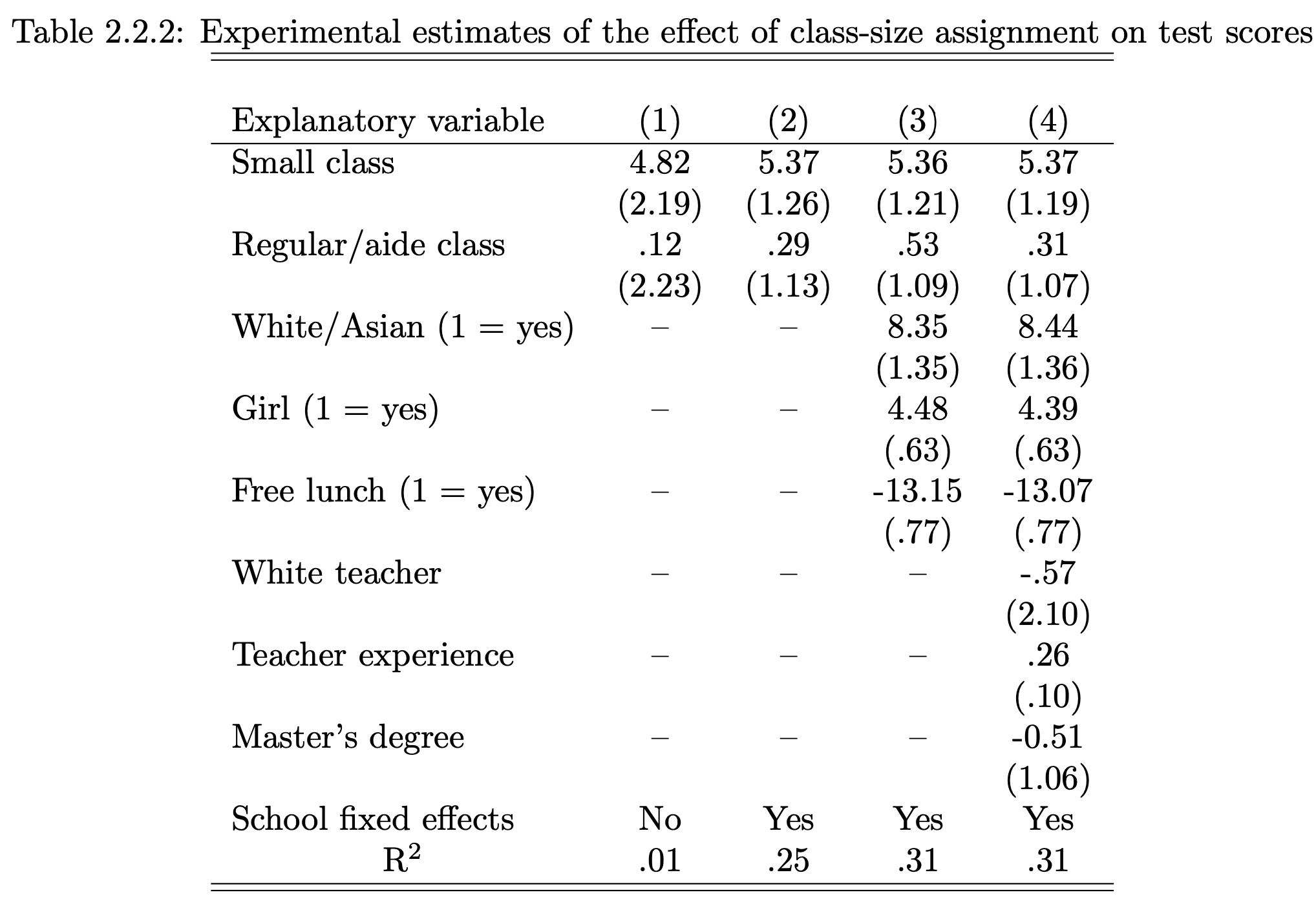
Table from Mostly Harmless Econometrics comparing estimated small-class effects across specifications with additional controls.

Source: Angrist and Pischke; retained from Unit 6, slide 26.

Discussion: what changes across columns?

Which coefficients are stable?
What happens to standard errors?
How can controls improve precision in an experiment?
What would a large change in the treatment coefficient prompt you to investigate?

Start with the table’s sample, units, and assignment process.

Omitted-variable bias

Suppose the population model is

$Y=\alpha+\beta X+\gamma Z+u,$

but we omit $Z$ . Under the usual exogeneity conditions,

$\operatorname{plim}\hat\beta_{\text{short}} =\beta+\gamma\frac{\operatorname{Cov}(X,Z)}{\operatorname{Var}(X)}.$

Both the outcome relevance of $Z$ and its association with $X$ matter.

Discussion: Jurajda

Choose one identification example from the notes.

Where does the relevant variation come from?
Why is a simple group comparison insufficient?
What institutional detail supports the design?
What alternative explanation remains?

Can you describe the ideal experiment?

Specify treatment, population, assignment, outcome, and follow-up period.

If the treatment itself is ambiguous, refine the question first.

Workshop: your identification statement

Complete:

“The relationship of interest is …”
“The ideal experiment would …”
“The feasible comparison is …”
“Its causal interpretation requires …”
“The largest remaining threat is …”

Before you leave

Explain why a precisely estimated coefficient can still answer the wrong causal question.

References

Angrist, Joshua D., and J"orn-Steffen Pischke. 2009. Mostly Harmless Econometrics: An Empiricist’s Companion. Princeton University Press.

Jurajda, Step’an. 2007. Lecture Notes on Identification Strategies. Lecture notes.

Timmins, Christopher, and Wolfram Schlenker. 2009. “Reduced-Form Versus Structural Modeling in Environmental and Resource Economics.” Annual Review of Resource Economics 1: 351–80. https://doi.org/10.1146/annurev.resource.050708.144119.